Handling Unwanted Contributions in Spectroscopic Data

Files

Ex_15_time_variant_unwanted_contributions.py

Ex_15_time_invariant_unwanted_contributions.py

Ex_15_multiple_experiments_unwanted_contributions.py

In many cases, there may be unwanted contributions in the measured spectra, which may come from instrumental variations (such as the baseline shift or distortion) or from the presence of inert absorbing interferences with no kinetic behavior. Based on the paper of Chen, et al. (2019), we added an new function to KIPET in order to deal with these unwanted contributions.

The unwanted contributions can be divided into the time invariant and the time variant instrumental variations. The time invariant unwanted contributions include baseline shift, distortion and presence of inert absorbing interferences without kinetic behavior. The main time variant unwanted contributions come from data drifting in the spectroscopic data. Beer-Lambert’s law can be modified as,

\[\mathbf{D} = \mathbf{C}\mathbf{S}^\top + \mathbf{G} + \mathbf{E}\]

where G is the unwanted contribution term.

The time invariant unwanted contributions can be uniformly described as the addition of a rank-1 matrix G, given by the outer product,

\[\begin{split}\begin{align} \mathbf{G} &= \mathbf{e}\mathbf{g}^\top\\ \mathbf{e} &= \left[1\;1\; \dots\;1\right]^\top_{(n_{tp} \times 1)}\\ \mathbf{g} &= \left[g_1 \; g_2 \; \dots \; g_{n_{wp}}\right]^\top\\ \mathbf{G} &\in R^{n_{tp}\cdot n_{wp}} \end{align}\end{split}\]

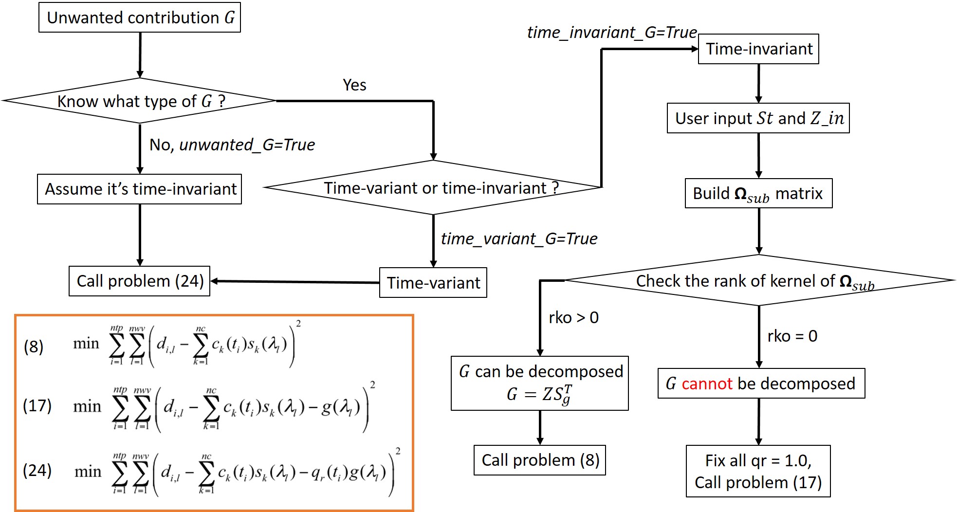
where the vector g represents the unwanted contribution at each sampling time. According to Chen’s paper, the choices of objective function to deal with time invariant unwanted contributions depends on the rank of kernel of Ω_sub matrix (rko), which is composed of stoichiometric coefficient matrix St and dosing concentration matirx Z_in. (detailed derivation is omitted.) If rko > 0, G can be decomposed as,

\[\begin{split}\begin{align} \mathbf{G} &= \mathbf{C}\mathbf{S}^\top_g\\ \mathbf{S}_g &= \left[\mathbf{s}_1^g\;\mathbf{s}_2^g\; \dots\;\mathbf{s}_{n_{wp}}^g\right]\\ \mathbf{S}_g &\in R^{n_{c}\cdot n_{wp}} \end{align}\end{split}\]

Then the Beer-Lambert’s law can be rewritten as,

\[\mathbf{D} = \mathbf{C}\left(\mathbf{S} + \mathbf{S}_g\right)^\top + \mathbf{E}\]

Thus, the original objective function of the parameter estimation problem doesn’t need to change while the estimated absorbance matrix would be S+Sg and additional information is needed to separate S and Sg.

If rko = 0, G cannot to decomposed. Therefore, the objective function of the parameter estimation problem should be modified as,

\[\begin{split}\sum^{n_{tp}}_{i=1} \sum^{n_{wp}}_{l=1} \left( d_{il} - \sum^{n_c}_{k=1} c_k(t_i)s_k(\lambda_l) - g(\lambda_l) \right)^2\\\end{split}\]

For time variant unwanted contributions, G can be expressed as a rank-1 matrix as well,

\[\begin{split}\begin{align} \mathbf{G} &= \mathbf{q}\mathbf{g}^\top\\ \mathbf{q} &= \left[q_1\;q_2\; \dots\;q_{n_{tp}}\right]^\top\\ \mathbf{g} &= \left[g_1 \; g_2 \; \dots \; g_{n_{wp}}\right]^\top\\ \end{align}\end{split}\]

and the objective of problem is modified as follows,

\[\begin{split}\min \sum^{n_{tp}}_{i=1} \sum^{n_{wp}}_{l=1} \left( d_{il} - \sum^{n_c}_{k=1} c_k(t_i)s_k(\lambda_l) - q_r(t_i)g(\lambda_l) \right)^2\\\end{split}\]

where the time variant unwanted contributions are considered as a function of time and wavelength. In addition, since there are no constraints except bounds to restrict qr(i) and g(l), this will lead to nonunique values of these two variables and convergence difficulty in solving optimization problem. Therefore, we force qr(t_ntp) to be 1.0 under the assumption that qr(t_ntp) is not equal to zero to resolve the convergence problem.

Users who want to deal with unwanted contributions can follow the following algorithm based on how they know about the unwanted contributions. If they know the type of the unwanted contributions is time variant, assign time_variant_G = True. On the other hand, if the type of the unwanted contributions is time invariant, users should set time_invariant_G = True and provide the information of St and/or Z_in to check rko. However, if the user have no idea about what type of unwanted contributions is, assign unwanted_G = True and then KIPET will assume it’s time variant.

Please see the following examples for detailed implementation. The model for these examples is the same as “Ex_2_estimation.py” with initial concentration: A = 0.01, B = 0.0,and C = 0.0 mol/L.

The first example, “Ex_15_time_invariant_unwanted_contribution.py” shows how to estimate the parameters with “time invariant” unwanted contributions. Assuming the users know the time invariant unwanted contributions are involved, information of St and/or Z_in should be inputed as follows,

St = dict()
St["r1"] = [-1,1,0]
St["r2"] = [0,-1,0]

# In this case, there is no dosing time.
# Therefore, the following expression is just an input example.
Z_in = dict()
Z_in["t=5"] = [0,0,5]

Next, add the option G_contribution equal to “time_invariant_G = True” and transmit the St and Z_in (if users have Z_in in their model) matrix when calling the “run_opt” method to solve the optimization problem.

r1.settings.parameter_estimator.G_contribution = 'time_invariant_G'
r1.settings.parameter_estimator.St = St
r1.settings.parameter_estimator.Z_in = Z_in

The next example, “Ex_15_time_variant_unwanted_contribution.py” shows how to solve the parameter estimation problem with “time variant” unwanted contribution in the spectra data. Simply add the option G_contribution equal to “time_variant_G” to the arguments before solving the parameter estimation problem.

r1.settings.parameter_estimator.G_contribution = 'time_variant_G'

As mentioned before, if users don’t know what type of unwanted contributions is, set G_contribution equal to ‘time_variant’.

In the next example, “Ex_15_estimation_mult_exp_unwanted_G.py”, we also show how to solve the parameter estimation problem for multiple experiments with different unwanted contributions. The methods for building the dynamic model and estimating variances for each dataset are the same as mentioned before. In this case, Exp1 has “time invariant” unwanted contributions and Exp2 has “time variant” unwanted contributions while Exp3 doesn’t include any unwanted contributions. Therefore, we only need to provide unwanted contribution information for each ReactionModel separately as you would for individual models.

Users may also wish to solve the estimation problem with scaled variances. For example, if the estimated variances are {“A”: 1e-8, “B”: 2e-8, “device”: 4e-8} with the objective function,

\[\min \frac{(D - C_A S_A - C_B S_B)^2}{4\times 10^{-8}} + \frac{(C_A - Z_A)^2}{1\times 10^{-8}} + \frac{(C_B - Z_B)^2}{2\times 10^{-8}}\]

this option will scale the variances with the maximum variance (i.e. 4e-8 in this case) and thus the scaled variances become {“A”: 0.25, “B”: 0.5, “device”: 1,0} with modified objective function,

\[\min \frac{(D - C_A S_A - C_B S_B)^2}{1.0} + \frac{(C_A - Z_A)^2}{0.25} + \frac{(C_B - Z_B)^2}{0.5}\]

This scaled_variance option is not necessary but it helps solve the estimation problem for multiple datasets. It’s worth trying when ipopt gets stuck at certain iteration.

kipet_model.settings.general.scale_variances = True