Background
This documentation focuses on kinetic studies for the investigation of chemical reactions and identification of associated rate constants from spectroscopic data. The methodology is the same as published in Chen, et al. (2016), where the technical details are laid out in significant detail. In this document the user will find a summary of the procedure in the paper as well as how this method has been transferred to KIPET. This document will therefore attempt to only describe as much detail as necessary in order to understand and use KIPET.
General modeling strategy and method
- After installing and importing the package users can do the following things:
Build a chemical reaction model
Simulate the model
Estimate variances in the data
Preprocess data
Perform estimability analysis
Estimate parameters
Ascertain whether a different subset of wavelengths is more suitable for the model
Compute confidence intervals of the estimated parameters
Plot concentration and absorbance profiles
This can be done for problems where we have multiple datasets from separate experiments or in the case of having concentration data only and not spectra.
The first step in KIPET is to create a model. A model contains the physical equations that represent the chemical reaction system dynamics. Once a model is created users can either make a simulation by solving the DAE equations with a multi-step integrator or through a discretization in finite elements. Alternatively an optimization can be performed in which the DAE equations are the constraints of the optimization problem. In general, KIPET provides functionality to solve optimization problems for parameter estimation of kinetic systems. For the construction of optimization models KIPET relies on the Python-based open-source software Pyomo. Pyomo can be used to formulate general optimization problems in Python. After a model is created users can extend the model by adding variables, equations, constraints or customized objective functions in a similar way to Pyomo. After the simulation or the optimization is solved, users can visualize the concentration and absorbance profiles of the reactive system. These steps are summarized in the following figure.
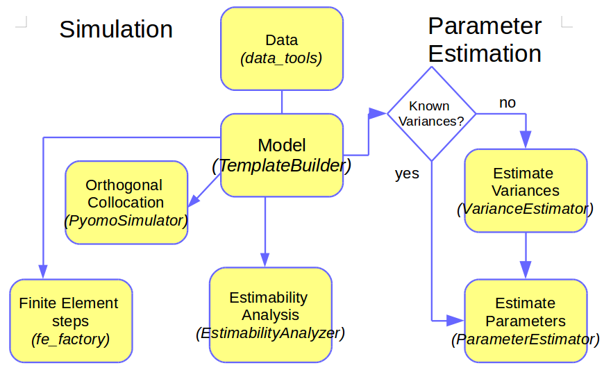
Fig. 4 The steps/modules involved in setting up a KIPET model
The variable nomenclature follows the same labeling structure as used in the original paper, Chen et al. (2016). Once the model is created it can be simulated or optimized. KIPET simulates and optimizes Pyomo models following a simultaneous approach. In the simultaneous approach all of the time-dependent variables are discretized to construct a large nonlinear problem. Due to the nature of large nonlinear problems, good initial guesses for variables are essential. KIPET provides a number of tools to help users to initialize their problems, including through the use of running simulations with fixed guessed parameters, using a least squares approach with fixed parameters, or through a finite element by finite element approach using KIPET’s in-built fe_factory (recommended for large problems and necessary for problems in which we have dosing). KIPET therefore offers a number of simulator and optimizer classes that facilitate the initialization and scaling of models before these are called for simulation. In addition, the simulator and optimizer classes available in KIPET will store the results of the simulation/optimization in pandas DataFrames for easy visualization and analysis. More information on this and why this is relevant to the user will follow during the tutorial problems. KIPET offers two classes for the optimization of reactive models. The ParameterEstimator class estimates kinetic parameters from spectral data by solving the problem formulation described in Chen, et al. (2016). Within this class the objective function is constructed with Pyomo and added to the model that is passed to the solver. If the user provides a model with an active objective function however, the ParameterEstimator will optimize the objective function provided by the user. This class also offers the ability to determine the confidence intervals of the estimated parameters. For all calculations in the ParameterEstimator class the variances of the spectral data need to be provided. When the variances are not known the user can use the VarianceEstimator optimizer class instead to determine them. We provide a number of different approaches to estimate the variances. The first one is the one described in Chen et al. (2016). The procedure consists of solving three different nonlinear optimization problems in a loop until convergence on the concentration profiles is achieved. The following figure summarizes the variance estimation procedure based on maximum likelihood principles:
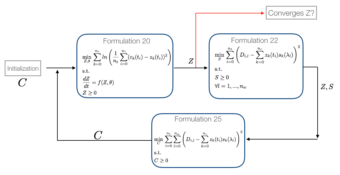
Fig. 5 The VarianceEstimator class algorithm 1 from Chen et al. (2016)
The VarianceEstimator class will construct the three problems and solve them with a nonlinear solver until the convergence criteria is satisfied. By default KIPET checks for the infinite norm of the residuals of Z between two iterations. If the infinity norm is less than the tolerance (default 5e-5) then variances are estimated by solving the overdetermined system shown in the next figure.
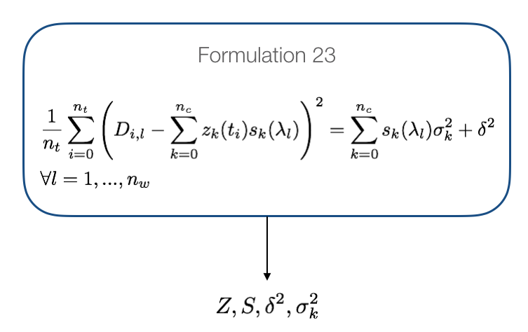
Fig. 6 Variance estimation equations
The solution of each subproblem in this procedure is logged in the file iterations.log. Examples on how to use the optimization classes and their corresponding options can be found in the tutorial section of this document. It should be noted at this point that all that is required to determine the variances in this way are the components, their initial concentrations, the differential equations describing the reactions, and the spectroscopic data absorption matrix, D, which consists of the experimental absorption data with rows (i) being the time points and columns (l) being the measured wavelengths. The above method was described in the initial paper from Chen et al. (2016). This method can be problematic for certain problems and so a new variance estimation procedure has been developed and implemented in version 1.1.01 whereby direct maximum likelihood formulations are solved. We propose and include 2 new methods as well as a number of functions in order to obtain good initial guesses for variance. The first and recommended method is known as the “alternate” strategy within KIPET. Here we solve for the worst-case device variance first:
where
Then we set:
We also know that, from derivations in Chen et al. (2016):
We guess initial values for σ (which the user provides) and solve the maximum likelihood-derived objective:
and then we are able to determine delta from:
Following this we can evaluate:
This function then provides us with the difference between our overall variance and the model and device variances. If the value of the function is below tolerance we stop or we update σ using a secant method and re-solve until we find convergence.
A third method is provided, referred to as “direct_sigmas” in KIPET, which first assumes that there is no model variance and solves directly for a worst-case device variance. The formulation solved is thus:
And from this formulation, the device variance can be solved for directly assuming that there is no model variance. Once the worst-possible device variance is known, we can obtain some region in which to solve for the model variances knowing the range in which the device variance is likely to lie. The following equation can be used to solve for different values of device variance:
Once these solutions are obtained we can solve directly for the model variances. A selection of model and device variances are then provided to the user, and the user is able to decide on the appropriate combination for their problem. More rigorous mathematical derivations of these methods will be provided in future documentation versions. Once the variances are estimated we not only attain good estimates for the system noise and the measurement error, but we have also obtained excellent initializations for the parameter estimation problem, as well as good initial values for the kinetic parameters to pass onto the ParameterEstimator class. Where Equation 17 from Chen, et al. (2016) is solved directly:
Note here that this can be solved either directly with the variances and measurement errors manually added and fixed by the user, or through the use of the VarianceEstimator. It is also important at this point to note that we can solve the ParameterEstimator problem either using IPOPT to get the kinetic parameters or we can use sIPOPT or k_aug to perform the optimization with sensitivities in order to determine the confidence intervals.